Sidebar
Table of Contents
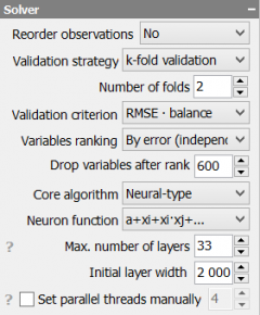
Solver
Solver module produces predictive models for target variables.
Reorder rows
Reorder rows is used to achieve uniform statistical characteristics of training and testing samples and to makes them equally informative. This technique works well for all problem types including time series models.
| Options | Description |
No | Reordering is turned-off |
Odd/even | Places all even instances after odd instances. Example: 1,2,3,4,5,6 → 1,3,5,2,4,6 |
Asc.+ Odd/even | Ascending sorting of observations (by target values) prior to Odd/even reordering. |
Desc.+ Odd/even | Descending sorting of observations (by target values) prior to Odd/even reordering. |
Validation strategy
Validation strategy is used to select a method for model validation and sorting out.
| Options | Description |
Training/testing | Splits dataset into two parts, uses the training part to find model coefficients and uses the testing part to compare and select a set of the best models. |
Whole data testing | Splits dataset, trains model using the training part, but uses both parts for testing |
k-fold validation | Splits dataset onto k parts, trains a model k times using k-1 parts, each time measuring model performance using a new remaining part. Finally residuals obtained from all testing parts are added and used for model comparison. |
k-fold training | In contrast to the k-fold validation, k-fold training uses k-1 parts to test the model and only 1 part to estimate coefficients. In other aspects it's similar to the k-fold validation. This is rather an extreme method that is used to stop over-fitting when other methods do not work. |
Leave-one-out CV | This is a k-fold cross-validation with the number of folds equal to the number of observations in the dataset |
Train/test ratio is used to split the dataset into training and testing part. Percentage or exact quantities are used. For example, if we would like to split a dataset containing 200 observations using the ratio 4:1, we can apply percentage 80:20 or exact number of observations 160:40.
Validation criterion
Defines model selection criterion for both the core algorithm and variables ranking.
Variables ranking
Variables ranking turns on preliminary ranking and reduction of variables.
| Options | Description |
No | Turned-off |
by error (independent) | Ranking of variables according to their individual ability to predict testing data |
by usage (combinatorial) | Ranking of variables according to their importance for Combinatorial Core algorithm with limited complexity (equal to 2). Importance is calculated as the number of times the variables appear in the set of best models. |
Drop variables after rank n
Reduces the number of variables to n i.e. keeps n most important variables according to the selected ranking algorithm. Preliminary reduction of variables may reduce the quality of models, but it is definitely useful for quicker processing of high-dimensional datasets.
Core algorithm
You can select one of the available statistical learning algorithms. The description of algorithms implemented in GMDH Shell can be found in Learning algorithms
| Options | Description |
Combinatorial | Best subsets regression, combinatorial search |
Neural-type | Polynomial neural networks of GMDH-type. |
Combinatorial
Limit Complexity to n
Any particular model may consist of not more than n terms.
Additional variables
Expands dataset with the new artificial features. Higher-dimensional space frequently helps to improve the Classification and Regression models. Be careful with expanding of more than 20 initial variables because the number of all possible pairs grows fast.
| Options | Description |
No | No additional variables except constant term. |
xi·xj | Adds all possible multiplied pairs. |
xi·xj, xj² | Adds all possible multiplied pairs and squares. |
xi·xj, xi/xj | Adds all possible multiplied and divided pairs. Skips pairs that cause dividing by zero. |
Custom | Uses terms of custom polynomial function as new variables, see Custom polynomial |
Be aware of quick growing of memory and time consumption.
| The number of initial variables | Resulting number of variables | |||
No | xi·xj | xi·xj, xi² | xi·xj, xi/xj |
|
| 2 | 3 | 4 | 6 | 5 |
| 3 | 4 | 7 | 10 | 10 |
| 5 | 6 | 16 | 21 | 26 |
| 10 | 11 | 56 | 66 | 101 |
| 20 | 21 | 211 | 231 | 401 |
| 50 | 51 | 1276 | 1326 | 2501 |
| 100 | 101 | 5051 | 5151 | 10001 |
| 200 | 201 | 20101 | 20301 | 40001 |
| 500 | 501 | 125251 | 125751 | 250001 |
Neural-type
Neuron inputs
The number of input variables allowed for a neuron. It is quite efficient to use two inputs for any neuron. Otherwise the computational task may become too complex.
Neuron function
Sets the type of the internal function for neurons. The neurons are active, i.e. each neuron can drop some of the function terms in order to increase overall predictive power of the model.
| Options | Description |
a0 + a1·xi + a2·xj | Linear |
a0 + a1·xi + a2·xj + a3·xi·xj | Polynomial |
a0 + a1·xi + a2·xj + a3·xi·xj + a4·xi² + a5·xj² | Quadratic polynomial |
Custom | Uses custom polynomial function defined by user, see Custom polynomial |
Max. number of layers
Sets the upper limit for the number of network layers created by the algorithm.
Initial layer width
Initial layer width defines how many neurons are added to the set of inputs at each new layer.
Set parallel threads manually
When turned-on, this option allows manual control of the number of parallel processing threads. When turned-off, the number of threads is equal to the number of logical processors i.e. processor cores or hyper-threading cores in your PC.
Custom polynomial
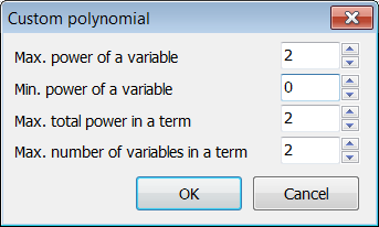
You can configure a Custom polynomial function to be used for generation of Additional variables or as a Neuron function. When the 'Custom' option is selected in the corresponding list of options, a dialog window called Custom polynomial is shown.
Max. power of a variable
Sets the upper limit for power of any variable in a polynomial term.
Min. power of a variable
Sets the lower limit for power of any variable in a polynomial term.
For example, if Max. power is 3 and Min. power is -2, then the following terms are included to the custom polynomial: x13, x12, x1, 1 (constant term), 1/x1, 1/x12. If Min. power is 1 or higher then resulting polynomial will not include a constant term.
Max. total power in a term
Sets a limit for sum of absolute powers of all variables in a polynomial term.
For example, if Max total power is 3 then the following terms can be included: x1*x22, x1*x2-2, x1*x2*x3, …
Max. number of variables in a term
Sets the maximum number of variables in any polynomial term. For example, if Max. number of variables is 3, then the following terms can be included: x1*x2*x3, (x12)*(x24)*(x3-1) …
Here are some configuration examples for two input variables:
Max. power = 2, Min. power = 0, Max total power = 2, Max number in a term = 2 results in:
y(x1,x2) = a0 + a1*x1 + a2*x2 + a3*x1*x2 + a4*x12 + a5*x22
Max. power = 4, Min. power = 0, Max total power = 4, Max number in a term = 1 results in:
y(x1,x2) = a0 + a1*x1 + a2*x12 + a3*x13 + a4*x14 + a5*x2 + a6*x22 + a7*x23 + a8*x24


