Sidebar
Table of Contents
Simulation results
Model browser
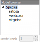
Model browser is used to select and browse simulation results of different target variables. Models are organized in a tree-like structure. Top-level nodes represent post-processed modeling results, while nested items represent one or more raw models.
When a raw model is selected you can use Model rank to access lower model ranks outperformed by the top-ranked model. One of the reasons for inspecting lower model ranks is that you can average them in the post-process panel.
Plot
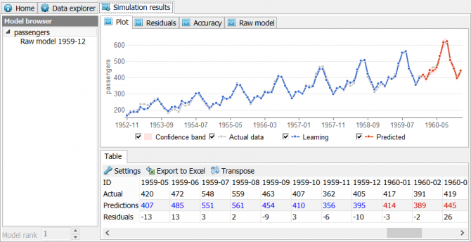
View > Simulation results > Plot is a time series chart used to analyse models visually. It is interactive like all other charts in GMDH Shell. You can view values, hold and move the curve, zoom chart, and save the chart to a file. When a model is selected in the Model browser the Plot outputs it immediately.
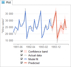
The chart has the following legend:
Predicted, i.e. model predictions are red.
Model fit are model values fitted to the data, they are blue.
Actual data, i.e. the data available from the initial dataset is gray.
Confidence band is the 95% confidence band calculated for predictions. Confidence band calculation uses model values fitted to the data (blue curve), it equals to two standard deviations (2*sigma) of model residuals.
If predicted values have no their own IDs or future timestamps cannot be automatically generated, the forecast values will be marked with +1, +2, +3 on the horizontal axes. The Plot outputs post-processed (final) predictions using a thick line with dots. Raw models are plotted with a thin line. Raw model plot is only accessible when a raw model is selected in the Model browser.
Raw model
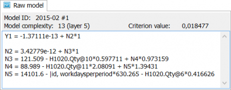
View > Simulation results > Raw model is used to view raw model selected in the model browser as an equation or a number of equations. GMDH Shell predictions are obtained after applying post-process transformations to raw model predictions.
Model ID informs which raw model is selected in the Model browser. The format is [model name][space]#[model rank].
Model complexity informs about the number of coefficients in the model and the number of layers. For example, 13 (layer 5) means the model has 5 layers and 13 coefficients.
Criterion value informs about the value of Validation criterion configured in the Solver module. Top-ranked model has the smallest criterion value.
Model formula
Model formula is one or several expressions that relate input variables and predicted variable. Each expression is composed from coefficients and input variable names. The names include one line transformations applied by the preprocessor, so they can be quite long. For example, model formula in the above screenshot contains the following variable names: “H1020.Qty@10”, “H1020.Qty@12”, “|id, workdaysperperiod”, “H1020.Qty@6”.
Accuracy
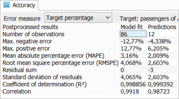
Accuracy is a panel accessible in the menu View > Simulation results > Accuracy that shows different accuracy metrics for the model selected in the Model browser.
Target shows the name of the model selected in the Model browser.
The table nested in the panel indicates in the upper left corner if it is the Raw model results or the Post-processed results. Other two header cells are Model fit and Predictions. The column Model fit contains accuracy measures calculated for observations used to crate the model. The column Predictions contains accuracy measures calculated for withheld observations, therefore if predicted values have no actual values this column is empty. Number of observations in the table informs about the number of actual observations both in the fitted and the withheld subsamples.
Error measure is used to choose a metric for calculation of the mean and the root mean errors. Available metrics are the Absolute, which outputs mean error values “as is”, the Range percentage, i.e. percentage of magnitude of predicted variable, and the Target percentage, where for each model value we calculate percentage deviation from the actual value and then the percentage deviations are averaged.
Calculation of predicted variable magnitude involves only the observations used for model training and testing.
| Error measure | Mean | Root mean square |
| Absolute | Mean absolute error (MAE) | Root mean square error (RMSE) |
| Range percentage | Normalized mean absolute error (NMAE) | Normalized root mean square error (NRMSE) |
| Target percentage | Mean absolute percentage error (MAPE) | Root mean square percentage error (RMSPE) |
Other accuracy measures available in the table:
Max. negative error, the largest underestimation
Max. positive error, the largest overestimation
Residual sum
Standard deviation of residuals
Coefficient of determination (R²)
Correlation coefficient
Importance
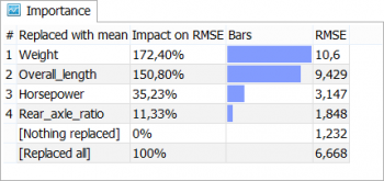
Accessible in the menu View > Simulation results > Importance the panel helps to understand the value of each input variable in a model.
To calculate importance of variables we replace variables in the model with their mean value one by one and measure the root mean squared error (RMSE) of the “new” model. Original model error is considered a zero percent impact on RMSE and 100% impact is a case where all variables are replaced with their mean.
The impact can easily exceed 100% in the case the variable in a model is multiplied by another variable or squared. A small negative percentage can also happen if a variable is merely useless for the model.
Importance table has the following columns:
Replaced with mean column contains the name of a variable tested by replacing with its mean value and two reference tests in the bottom of the list.
Impact on RMSE is a percentage value that helps to compare variables and reference values, it is calculated as
Impact = (R_var - R_ori)/(R_all - R_ori)*100%
where R_var is RMSE of the variable we consider, R_ori is zero-impact RMSE and R_all is RMSE of a model where all variables are replaced with mean.
Bars column visualises difference between the variables.
RMSE is a root mean square error obtained for the model in a result of the importance test.
Table
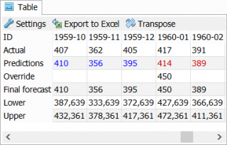
Table is a panel accessible in the menu View > Simulation results > Table, it is used to output simulation results shown in the Plot as a table of numeric values.
Table has a toolbar with tree buttons:
Settings button opens the Settings dialog box.
Export to Excel exports the table to Excel spreadsheet located in the project directory.
Transpose button changes table arrangement from vertical to horizontal and vice versa.
Settings
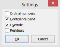
Settings is a dialog box accessible via the Settings button in the panel toolbar. The dialog box is used to configure the output of the table.
Ordinal numbers adds enumeration of observations and predictions to the table with the heading #.
Confidence band adds Upper and Lower margins of the confidence band.
Override is used to change predicted values manually by typing into the Override cells.
Residuals is used to add differences between actual and model values. If the model operates with categorical targets, residuals are replaced with Hit and Miss marks.
Other entries of the table are:
ID values are unique identifiers or timestamps.
Actual values are actual values of target (predicted) variable.
Predictions are post-processed predictions of the target variable.
Raw model heading and values replace Predictions in the table if a Raw model is selected in the Model browser.
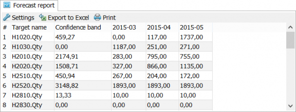
Forecast report
Forecast report accessible in the menu View > Simulation results > Forecast report contains forecast of all target variables in one table.
You can use the configuration button to change appearance of the report. Also, you can save the report to XLS file or print. To save the report in the PDF, you should use a third party virtual PDF printer.
Inventory report
Inventory report is accessible in the menu View > Simulation results > Inventory report. It is used to generate purchase orders for inventory replenishment.

The report aggregates demand forecast calculated by GMDH Shell, inventory replenishment information and warns about potential stockouts and overstocks.
There are four sections in the table: Inventory, Replenishment calculation, Forecast by periods and Identified issues.
Inventory section shows available information about the stock: Description of the items and the Item code.
Replenishment calculation shows information for planning the replenishment of the stock:
- On heands - the available product stock; is read from the “!inventory.xls” file.
- Lead time - the time (in months) between the placement of an order and delivery. Is read from the file “!inventory.xls” if it exists, otherwise the default value of “1” is applied to all the items. The default value can be changed in the report settings via the Settings button found above the table. You can also edit the value directly in the table. All the values edited by a user appear in a blue color in the table.
- On order - the number of already ordered units of the item. Is red from the “!inventory.xls” file.
- Min order - the minimal item quantity that is required in the order. Is read from the “!inventory.xls” but can be edited manually by a user.
- Safety stock is an assessment of the reserve stock for the next lead time period in which there are no stockouts according to the forecast. The assessment can be calculated using one of the three methods chosen in the report settings. To specify the method click the Settings button.
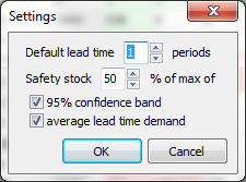 The safety stock can be calculated as given percentage taken from the:
- confidence limit;
- averaged sales volume over the past lead time period;
- maximum of the methods mentioned above.
You can also set the value manually.
- To order is the quantity that should be ordered according to Forecast by periods, Lead time, inventory On hands, On order, Safety stock, Min order and calculated as follows:
To_order = {min(0; Fn + Safety_stock - min(0; On_hands + On_order - Fc)) }Min_order,
where the:
FnandFcare the summed forecast over the next and the current lead time period correspondently;min(a; b)returns the minimum among theaandb;{v}Min_orderrounds thevto the nearest upper value that is multiple of Min order.
Cells in the Forecast by periods section are colored with green and red colors. The green cells show how many periods you are able to sale using the resources of the On order and On hands cells. Periods with shortages are red.
The Stockout column in the Identified issues section says about the amount of shortage in the current lead time period. It is calculated for the items having red cells as:
Stockout = |On_hands + On_order - Fc|.
The Overstock column indicates the products that are overstocked in the next lead time period. The values are calculated for the items having only green cells as:
Overstock = On_hands + On_order - Fc - Fn - Safety_stock.
Toolbar
Default lead time is used to set the lead time for all items that have no lead time information in the Inventory section of the Inventory report.
Export table is used to export the whole Inventory report to a spreadsheet.
Export order is used to export the items and quantities that have to be replenished.
~~UP~~

