An important task of any production company is to plan its manufacturing forces according to the future market demand. GMDH Shell BF was designed to help in two vital areas of every business: demand forecasting and inventory replenishment. This section concentrates on the first one and will guide you through a sample forecasting session in terms of the basic forecasting workflow. We will consider forecasting the demand on products for some general-purpose store.

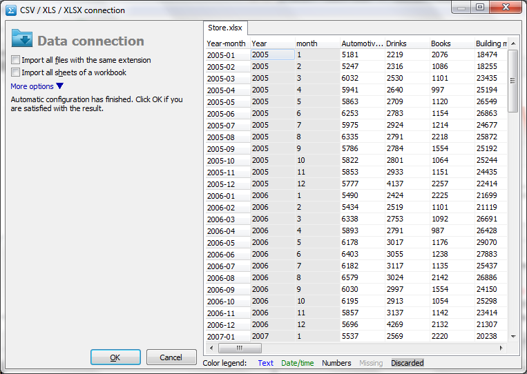
Let us create a new project by clicking the New toolbar icon. The sales data stored in an Excel file format, so choose CSV/XSL/XSLX connection. Select then the file Store.xlsx and click Open. This will call up the file connection dialog shown in the figure below.

Right side of the dialog enables you to preview, how exactly the data of the file will be read. You can see the table, where the data of every column represent sales of some SKU and the row headers depict the sale dates. GMDH Shell BF automatically detects:

• any rectangular data table, whatever row or column format is used;
• column labels;
• time stamps columns like year, month, day, time and sets it as one ID column or row header (on the figure below the columns that combined in ID column are in gray).

To be processed properly, the data table should be read as shown below: a variable (SKU) occupies a single column in the preview table. If automatic detection can’t get this result, click More options link, and adjust connection options manually. These options described in the Data Connection section of the reference.

Click OK.

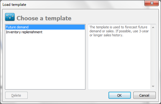
GMDH Shell BF now offers us to choose the template.

The software has to build-in templates purposed to the following problems: demand forecasting and stock replenishment based on the forecasts. We recommend using as more data history as you can collect. If possible, use at least 3-year sales history to get reliable enough forecasts. Our data file contains nine-year sales history so that’s sufficient enough. Select the first one and click OK.

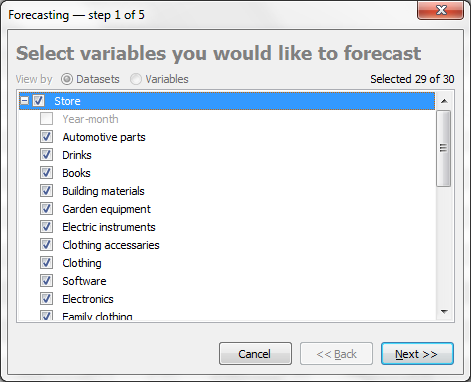
After the template has been set, the Wizard is started. It’s designed to help you to specify all the options and data used to generate forecasts. The first step is to select the variables you want to forecast.

Let us need to forecast them all. Select them and click Next.

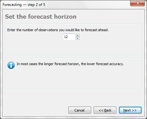
Forecast horizon defines the number of observations, you want to forecast ahead. It may range from minutes to years, depending on the data discrecity and the available volume of data. Nevertheless, it is recommended the horizon be no more than 25% of the number of observations. Otherwise, the results tend to have lower accuracy and be less reliable. Let we need to get a sales forecast for a year ahead. Since the data are monthly, type in “12” and click Next.

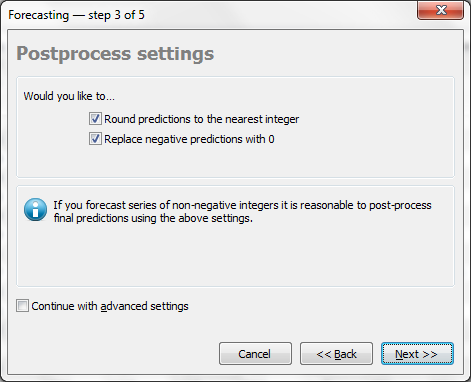
GMDH Shell BF offers to round obtained forecast to the nearest integer and make them nonnegative. These options make sense in most cases in sales forecasting. If you forecast things counted in integers it would be reasonable to leave the first option checked. The second option usually left checked but the case when you need to forecast returns too. We leave these options checked and click Next to start generating the forecasts.

Continue with advance settings option allows you to: 1) specify input variables that will be used for forecasting; 2) adjust the computational volume of processing.

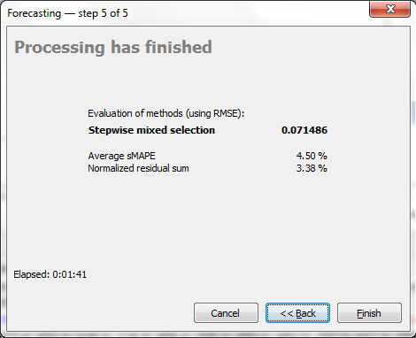
Once the processing has finished GMDH Shell BF shows an accuracy report for the Stepwise mixed selection forecasting method. The evaluation is based on the holdout approach and presented by the RMSE value.

The average accuracy over all forecasted SKUs is shown via sMAPE (the first formula on the page) and the NRS (normalized residual sum):

Where n is the holdout data set length, ya,i and yf,i are the actual and forecasted values in i-th time point.

Firstly, the Wizard splits the data series into two parts: learning part and holdout part. Then it runs a series of simulations to find the learning set length, which gets the best forecasting accuracy. Finally, the Wizard evaluates the forecasting method using the holdout part of the data. On the figure above the Stepwise mixed selection method was evaluated.

Notice that the Wizard acts in much the same way as an expert statistical analyst. It performs a series of tests, interprets the results, evaluates the forecasting method, and finally makes recommendations based upon the results.

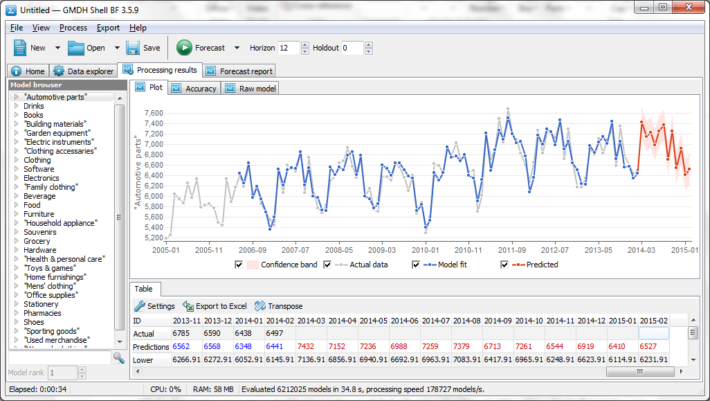
After you click Finish, GMDH Shell BF applies the forecasting method to the data to build the forecasts. The Processing results tab, having the Model browser, the Plot, and the Table panels, is now activate. Model browser contains a tree where the first level nodes are the forecasted items. The Plot and the Table display the information of currently selected item in the Model browser (see figure below).

All the forecasts were generated basis on the models built using the Wizard.

Let’s now explore some of the graphical options. The gray line on the graph represents the demand history of the Automotive parts, so that’s the actual data. The blue line is the model response on the learning part of the data. These data used to build the model. The red line is the forecast. And the light red area around the forecast is the confidence zone limited by [-2σ; 2σ] interval that should cover 95% future model errors. The checkboxes below the plot hide or show the corresponding data on the plot.

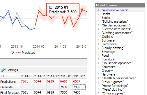
To see the numeric value of the point on the plot, move the cursor to the point and hold a little, the data will be showed up.

Let’s zoom in the data of the last three years and the forecast. To select this area, click left mouse to create the left-top corner of the rectangle (the cursor takes the form of a cross) and move the mouse to desired right-bottom point holding the button. The selected area will be outlined by dotted line (see figure below). Finally, release the button.

If you need to move the zoomed frame across the plot, click and hold the right mouse button (the mouse cursor takes the icon) and move the cursor in the desired direction.

There are two ways to zoom the plot out:

• do the same actions as we did when zooming in, but the bottom rectangle corner should be left-oriented;
• call up the plot context menu by clicking right mouse button on the plot and select Zoom out.

The first way is seemed to be handier.

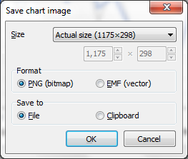If you need to copy the plot to the clipboard or to save it on your hard disk, you can again use the plot context menu. Call it up and select Save image….

Specify the image size using the Size option. There are some predefined variants and you can set your own. Choose then the format (vector or bitmap). Finally, choose the destination: file or clipboard.

You can also work with the plot in a full screen mode through the Full screen command from the plot context menu. To exit from the full screen mode, press the Esc button.

The Table of the Processing results tab displays the information depicted on the Plot numerically. By default, the Table is horizontally oriented, but you can change that using the button Transpose located above the Table.

Let’s take a closer look at the Table. The ID row contains the timestamps or the ordinal numbers of the observations if the timestamps are absent. The Actual row is populated with the historical data of the item selected in the Model browser panel. The model response and its forecast are in the Predictions row. Upper and Lower rows depict confidence limits of the [-2σ; 2σ] interval. The Overriding row is purposed to make manual adjustments to the statistical forecast. The end forecast is then depicted in the Final forecast row.

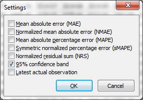
To customize rows of the Table, click the Settings button above the Table. The settings dialog allows you to show or hide such information as:

• Ordinal numbers. Additionally to timestamps shows the ordinal numbers of the observations. If the timestamps are absent, the ordinal numbers are shown instead automatically.
• Confidence band. Shows the confidance are of the forecast.
• Override. Shows override row allowing making manual adjustments to the forecast.
• Residuals. Shows the differences between corresponding values in the Actual and the Predictions rows.

There will undoubtedly be times when you want to judgmentally override the statistical forecasts. For instance, you may know of a large incoming order and need to change a number or two. GMDH Shell BF allows you to make these changes quickly and easily through the Overriding row of the Table.

Let us know that the forecast for the Automotive parts for the first two months of the 2015 year will be 7500 and 7400 accordingly. Just put the cursor on the certain cell in the Overriding row and type-in the value. The Plot and the Final forecast row will be updated immediately.

All overridden items are marked with blue color in the Model browser.

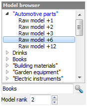Model browser allows you to select certain forecasted item. It contains a tree where the first-level nodes are the forecasted items. If the number of items is too large you can quickly find and select the certain item using the search field found above the tree. Type-in the item name and click search icon or press Enter.

First-level nodes of the tree represent the model response after the post-processing. The second-level nodes represent raw models which are used to create an overall picture that you see on the Plot when the parent (first-level) node is selected.

The number, prefixed with the “+”, in the raw model name indicates the forecast horizon of the raw model. Despite that the forecast was built for the 12 months ahead, you can see just five raw models in the figure below. The fact is that some of them used to create forecast more than for one time point.

Let’s select the raw model used to build a forecast for sixth time point. The Plot displays its response with the thin line while only the points of the model (parent node) response are displayed. The Predictions row is replaced with the Raw model one, the Lower, the Upper and the Override rows are cleared and the Override one is blocked in the Table. The Raw model row now displays the raw model response in numeric format.

Notice, that as you select a raw model in the Model browser, the Model rank option is enabled. To build every raw model a number of competitive variants are compared. A certain amount of the best of them are stored. These submodels are ranked by minimum of their error obtained on the learning part of the data. The Model rank option allows you to select these competitors, and the Plot and the Table – to show information about them.

Let’s take a closer look at the Forecast report tab.

Here is a table comprising point forecasts for all the items forecasted. It also includes the Confidence band column, representing the range forecast through the two-sigma confidence interval.

The columns of the table can be customized via the Setting button located above the table. These settings allow viewing model errors (MAE, NMAE, MAPE, sMAPE and NRS) on the holdout data set.

Forecast generation uses all the available data, thus there is no holdout set and these errors cannot be calculated; if you turn on these checkboxes and click OK, the respective table columns will be empty.

Exporting the results from the GMDH Shell BF to the other software such as Excel or saving them in a text file is one of the most frequently used commands.

GMDH Shell BF provides a number of exporting procedures, including exporting forecasts, predictions, model’s formula and its values. Exporting can be performed for the concrete forecasted item as well as all items at once.

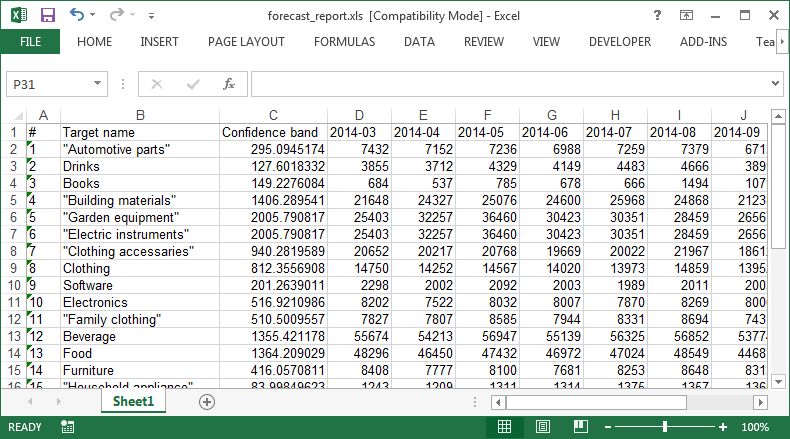
To export the forecasts of all the processed items in Excel file, go to the Forecast report tab and click on the Export to Excel button found above the forecast report table. The entire table will be copied into a new Excel file and automatically saved of “forecast_repotr.xls” name. The file will be saved in the directory where the input data is located.

The predictions of a particular item can be saved using the toolbar of the Table tab. Select the item in the Model browser panel, click then on the Export to Excel button of the toolbar. The table will be created in a new Excel file, having the columns Predictions, Final forecast, Override and so on. The file is automatically stored of the “!table.xls” name. If a file named “!table.xls” already exists in the data file directory, it will be replaced.

The final step is to save our current forecasting session as a project. Saving a forecast project allows you to return later and pick up where you left off or to share the session with others. Click on the Save button of the program toolbar or select File > Save project and save the project using the ‘Demand forecasting’ name.

Exit the program.