User Guide
1. Streamline Client
2.Streamline Server
3. Starting Up
4. Connecting data
5. Demand and Sales Forecasting
6. Inventory Planning
7. Reference
1. Streamline Client
2.Streamline Server
3. Starting Up
4. Connecting data
5. Demand and Sales Forecasting
6. Inventory Planning
7. Reference
 Add this page to your book
  Remove this page from your book
 The formulas below refer to calculation an ordering plan for planning items that are not distributed in DCs. In other words, demand for these planning items is generated by selling activity, not distribution. Ordering plan calculation for planning items that are distributed is described in the Two-echelon planning article.
To calculate the first planned order, Streamline uses the following Excel-like formula:
Order qty1 = MAX(CEILING(MAX(0, DOC + Safety stock + Qty_to_shipLT,OC - Remaining), Rounding), Min lot) (1),
Remaining = MAX(0, MAX(0, On hand) + Qty_to_receiveLT,OC - DLT),
where:
The calculated Order qty1 is shown in the Qty column of the Current order section on the Inventory planning tab.
To calculate replenishment orders for the next order cycles, the following Excel-like formula is used:
Order qtyi = MAX(CEILING(MAX(0, D(OCi) + Safety stocki + Qty_to_ship(OCi) - Qty_to_receive(OCi) - Remainingi-1), Rounding), Min lot), i = 2,…, (2)
where:
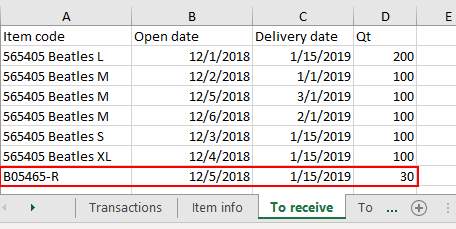
i-th Order cycle period.i-th Order cycle period.i-th Order cycle period.To demonstrate how Streamline calculates an ordering plan, we will use the built-in example Inventory Planning by Month. We have slightly changed the input data of the project:
As we mentioned above, an ordering plan is calculated in two steps. First, the current order quantity is computed.
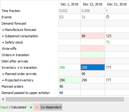
To figure out how the current order of 96 units is obtained, we will address the Explain inventory calculation dialog. To open it, we set the cursor at item B05465-R and press Ctrl + E (see figure below).
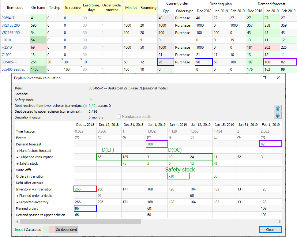
As Lead time = 10 days that ends up on Dec 12, 2018 and the Order cycle is 1 month, we take the Subperiod consumption demand starting from the end of Dec 12, 2018 to the end of Jan 12, 2019. Since the dialog shows the dates the particular subperiod ends, we take the sum for the four subperiods staring from Dec 31, 2018.
Now, let's replace the parameters with the values:
Order qty1 = MAX(CEILING(MAX(0, 162 + 94 + 30 - 200), 12), 60) = 96,
Remaining = MAX(0, MAX(0, 266) + 0 - 66) = 200.
We highlighted the values that are used in the calculation of the Current order quantity with positive and negative signs via green and red borders correspondingly in the figure above.
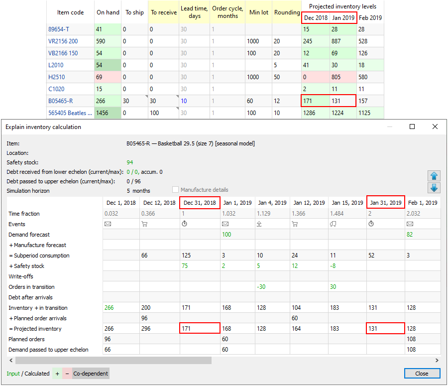
The values for all of the parameters in the formula (2) can be directly found in the Explain inventory calculation dialog as well. The most interesting from them is the Remainingi-1, i = 2,… . The Inventory + in transition row shows these remainings. The figure below highlights the values of the parameters that are used to get the second order.
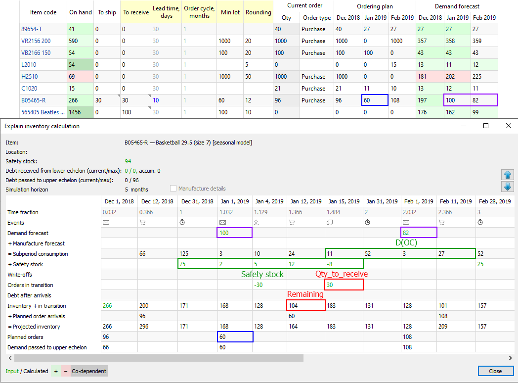
We have intentionally set Streamline to determine safety stock as the demand for the given number of future periods (1 month in our example) to be able to show you how the order amount is calculated.
Now, let's replace the parameters with the values:
Order qty2 = MAX(CEILING(MAX(0, 93 + 84 - 30 - 104), 12), 60) = MAX(CEILING(43, 12), 60) = 60.
To calculate the ordered quantities correctly in these more generic cases, the formulas (1) and (2) should account for the values from the mentioned rows.
To find out how the future on-hand levels at the end of each period are calculated, we will use two rows of the dialog table, Inventory + in transition and Planned order arrivals.
If you set the cursor at any cell of the Inventory + in transition row, you'll see the cells taking part in the calculation of the value. This row calculates the remaining on-hand at the end of each subperiod based on the:
In other words, this row shows on-hand remaining at the end of each subperiod without taking into account Streamline's deliveries (the Planned order arrivals row). The resulting projected inventory levels, which is the sum of the Inventory + in transition and Planned order arrivals rows, are indicated in the Projected inventory row. Consequently, the amounts at the end of each data aggregation period in this row make up the Projected inventory levels report (see figure below).
 Manage book (
 Help
Help