User Guide
1. Streamline Client
2.Streamline Server
3. Starting Up
4. Connecting data
5. Demand and Sales Forecasting
6. Inventory Planning
7. Reference
1. Streamline Client
2.Streamline Server
3. Starting Up
4. Connecting data
5. Demand and Sales Forecasting
6. Inventory Planning
7. Reference
 Add this page to your book
  Remove this page from your book
 The Panel of the Demand forecasting tab contains a set of properties and settings for forecasting, inventory planning, and key performance indicators. These properties and settings are set and displayed for the currently selected node in the Tree view. The Panel consists of the following tabs:
The Forecasting tab holds options used as input information in the forecasting model building process. All the forecasting settings can be applied on an item, category or location level, generally, at every level of the tree. To put these settings into effect, re-forecast the project by clicking the Forecast button.
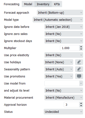
Here is the list of the forecasting settings:
The Forecast approach control has the following options:

This option is helpful if you need to apply Top-down method to a huge set of categories and use the Bottom-up approach for the item on the top of them.
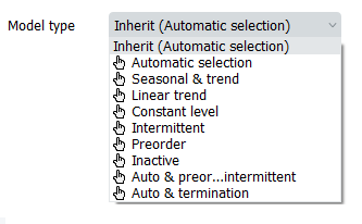
The  Model Type gives access to manual selection of forecasting models. There are several options:
Model = (Level + Slope * Time) * Seasonality
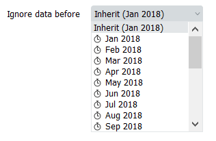
 Ignore data before control allows reducing the item’s sales history that is used to build the forecasting model. All the periods before the selected period are ignored. Data of the selected period is used to build the model. This option is helpful when you need to use a shorter length of history. For example, when sales volume has changed its level recently due to significant price change.
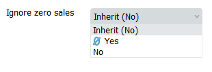
 Ignore zero sales
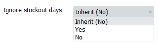
Ignore stockout days:
 Multiplier. The result of the model will be multiplied by the multiplier. This option is used to increase or decrease the model output.
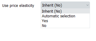
Use price elasticity
Feature considers not only qty sold in the past to generate a forecast but also notices the connection between an increase or decrease of sales and price change.
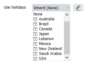
 Use holidays enables taking into account holidays of the given calendar when Streamline is building the model for the item.
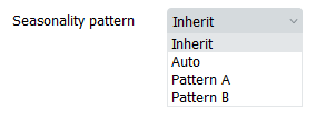
Seasonality pattern Allows to work with existing seasonal patterns or create new ones. For more see Seasonality pattern article.
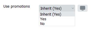
Use promotions Feature considers promotions imported from data source. As for now, Streamline supports only percentage discount promos and in order for the feature to work, you need to have at least one promotion in the past and one for the future period.
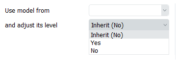
Use model from
Allows to copy a forecast from one item and apply it to another. Mostly used for brand new items if a similar item already exists on the market.
and adjust its level allows adjusting the level of the borrowed forecast to the level of the actual sales of the new item.
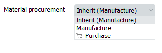
 Material procurement parameter allows you to enable/disable manufacturing for the particular node of the data tree. This option gets into the action if bill of materials was imported.
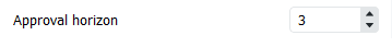
 Approval horizon is a time fence feature that allows to lock forecast of approved time periods.
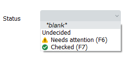
Status control helps you to set which forecasts are satisfied or need to be revised in the future. The control differs in the set of options whether a tree leaf or branch is currently selected. If a tree leaf is selected it has the following options:
 Needs attention. This is a kind of reminder that is set when you are not sure which forecast correction to make at this time and have decided to make it later. An attention icon is added to the node and all the nodes above it to easily spot such items if the tree is collapsed. This status stays with the item whatever changes we made to the item's model in the Model tab.
The Model tab shows the name of the model type chosen for the item, as well as the forecasting model structure and its coefficients in the table. Also, there’s a button “Save as pattern” that allows a user to save a particular set of coefficients to then apply that seasonality to another item. Read more.
You can adjust each of the coefficients of the model to align the forecast with your needs. Alternatively, to change the forecast, you can use the forecast overrides. Information on this tab is available only for the tree leaves. There are two types of models in Streamline, the time-series model and the intermittent demand model.
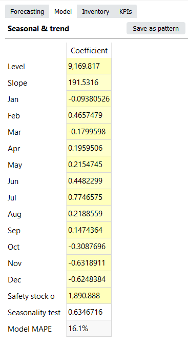
Generally, the model looks like:
An example of the time-series model is shown in the figure on the right. All cells with the yellow background are editable in Streamline.
An example of the time-series model is shown in the figure on the right. All cells with a yellow background are editable in Streamline.
Calculation of the forecasts
The exact formula to calculate the forecast for a period is:
,
,
.
Where:
i is the number of the forecasted period;Nblue is the number of blue points in the Plot;seasonal coefficient is the seasonal coefficient of the month of i-th period. For weekly model, the seasonal coefficient is a linear combination of seasonal coefficients of two adjacent months; andholiday coefficient is a holiday coefficient that falls to this period.Example
Consider an example of forecast calculation. We will use the build-in Streamline example of Multi-location Demand and Revenue Forecasting having monthly data.
Let’s take a look at the first item 00266-1 in the East location, and change the model Slope from 0 to 1.5 for demonstration purposes.
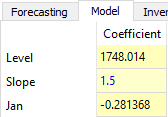
The model is built based on fourteen periods from November 2015 to December 2016. The forecasts of this model range from January 2017 to December 2017:
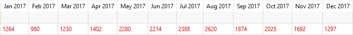
Let’s calculate the forecast for January 2017. It’s the first forecasted period, thus i = 1.
Jan_2017 = (1748.014 + 1.5 * ( (14 - 1) / 2 + 1) ) * (1 - 0.281368) = 1264.26
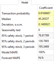
Several criteria trigger the intermittent demand model in Streamline. One of them - when a part of zero demand periods exceeds 60% of demand history length.
This model always returns ‘0’ as expected sales, but calculates Safety stock based on stochastic model of log-normal distribution. That is, the intermittent demand model expects that a log-normally-distributed transaction occurs with a probability of p, and no sales with probability 1-p.
The Median, Deviation, and Transaction probability are the parameters of the distribution which are estimated. Alternatively, you can set them manually in the Model tab.
The Deviation is given in orders of magnitude (o.o.m.). One order of magnitude is 10 times greater/less, so Deviation is usually very small.
There are three calculations for the item safety stock right below the Seasonality test row. The first one shows Safety stock calculated for one future period based on service level of 95%. The second one, for two periods. And the last one, for three periods. As you see, the more periods safety stock covers, the larger it supposes to be.
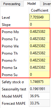
This model comes into play if the forecasted item has information on promotions imported and the data aggregation period is one week.
The promotional model is characterized by seven additional coefficients describing the future promotions weight into the generated forecasts (see figure on the right). Each of the coefficients corresponds to a particular day in the week.

The Inventory tab shows most of the columns of the Inventory planning tab. The table below shows a description of them.
| Property | Description |
|---|---|
| On hand | Shows the current item on-hand quantity in stock |
| Days of supply | Shows how many days of the future demand, starting from the project date, the current On hand (including orders to ship) can cover |
| To ship | Shows the total quantity on open sales orders and backorders |
| To receive | Shows the total amount on open purchase, transfer, and manufacturing orders |
| Lead time | Shows the interval of time between transfer/purchase order placement and its receipt |
| Order cycle, months | Shows how often the item is ordered from the supplier or distribution center |
| Min lot | It is the minimum quantity of the planning item that you can order from your supplier or distribution center |
| Max lot | It is the maximum amount of the planning item that you can order from your supplier or distribution center |
| Rounding | It is a constraint that rounds the Net order amount up to the given quantity |
| Service level, % | It is the percentage of the time (in the long run) that the item is available in stock |
| Safety stock | Indicates the safety stock for the planning item |
| Shelf life, months | It is the desired time the item can be in stock |
| Shelf life exceeding | It shows the average percentage of the current order quantity that we might have to discard |
| Sales price | Shows the current sales price/unit for the planning item |
| Purchase price | Indicates the price you pay the supplier for the item in the supplier's currency |
| Inventory value/unit | Shows the balance value of one unit of the item in stock imported from your data source |
| Gross margin | Shows the gross profit margin of the planning item |
| Turn-earn index | Indicates the item gross margin accumulated over the last 12 months |
| Current order | It is the recommended quantity to order currently |
| Value | Shows the value of the current order quantity in the supplier's currency |
| Stockout | It is the maximal expected inventory shortage during the Lead time period |
| Overstock | Shows the expected inventory level at the end of the Lead time plus Order cycle period |
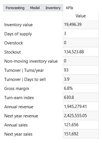
The KPIs tab shows important performance indicators of the item.
 Manage book (
 Help
Help